5. Segment and quantify#

This is the one that pays for the previous four. We take the raw time-lapse, segment every cell with a deep-learning model, measure them in physical units, throw out the artefacts, and end with a growth rate — the kind of number that goes in a figure.
Notably, none of this needs tracking. extract_growth()
aggregates cell area per timepoint, so you get a population growth rate from
segmentation alone. Tracking is what you add when you want per-lineage
answers.
Tip
No GPU required. Omnipose’s bact_phase_omni is a small model — the whole
notebook runs in about a minute on a plain CPU, so it works on a laptop or a free
Colab runtime. A GPU makes it faster, not possible.
# On Colab (or any fresh environment) this installs acia.
# Locally, if you already have acia installed, it is a no-op.
try:
    import acia  # noqa: F401
except ImportError:
    %pip install -q acia
Install a segmentation backend#
We use Omnipose with its bact_phase_omni model, which is trained on exactly
this kind of imagery: bacteria in phase contrast. It is also small (a 25 MB
model) and fast enough on a CPU that this notebook runs without a GPU in about a
minute.
acia supports several backends, but they pin conflicting versions of
cellpose, torch and numpy, so exactly one can be installed per
environment — see Installation. Swapping backends is a one-line change
in the cell further down; swapping environments is the price.
try:
    import omnipose  # noqa: F401
except ImportError:
    %pip install -q omnipose==1.0.6 natsort
from pathlib import Path
from urllib.request import (
    HTTPBasicAuthHandler,
    HTTPPasswordMgrWithDefaultRealm,
    build_opener,
    install_opener,
    urlretrieve,
)

# A public ownCloud share. The share token acts as the username, so single
# frames can be fetched over WebDAV instead of downloading the whole 800-frame,
# ~800 MB archive.
SHARE = "D0A9ftcpqwKm1Rq"
BASE = "https://fz-juelich.sciebo.de/public.php/webdav"
SEQUENCE = Path("data/colony")

N_FRAMES = 20  # of 800 available
FRAME_STEP = 20  # every 20th frame -> 20 minutes between the frames we keep

mgr = HTTPPasswordMgrWithDefaultRealm()
mgr.add_password(None, BASE, SHARE, "")
install_opener(build_opener(HTTPBasicAuthHandler(mgr)))

SEQUENCE.mkdir(parents=True, exist_ok=True)
for i in range(N_FRAMES):
    name = f"t{i * FRAME_STEP:04d}.tif"
    target = SEQUENCE / name
    if not target.exists():
        urlretrieve(f"{BASE}/00/{name}", target)

print(SEQUENCE, "->", len(list(SEQUENCE.glob("*.tif"))), "frames (~1 MB each)")
data/colony -> 20 frames (~1 MB each)
Load the sequence#
We work with all 20 downloaded frames at full resolution — Omnipose is cheap enough that there is no need to shrink further here. On a longer sequence, or a heavier backend, the subsampling habit from tutorial 2 is what keeps iteration fast.
import torch

print("accelerator:", "cuda" if torch.cuda.is_available() else "none (CPU)")
print("Omnipose runs fine either way -- roughly 3 s per frame on a CPU.")
accelerator: none (CPU)
Omnipose runs fine either way -- roughly 3 s per frame on a CPU.
from acia import ureg
from acia.segm.open import open_sequence

src = open_sequence(SEQUENCE).position(0)
src = src.with_pixel_size(0.072 * ureg.micrometer).with_frame_interval(20 * ureg.minute)

print(f"{len(src)} frames, {src.size_h}x{src.size_w} px")
print("time span:", src.timepoints[-1].to("hour"))
20 frames, 1094x938 px
time span: 6.333333333333333 hour
Segment#
A segmenter is a callable: hand it a source, get back an
Overlay of detections. The model is loaded lazily on first
use and, by default, released afterwards so the GPU memory goes back to the
system.
from acia.segm.processor.omnipose import OmniposeSegmenter

segmenter = OmniposeSegmenter(model="bact_phase_omni")

overlay = segmenter(src)

print(len(overlay), "detections across", overlay.numFrames(), "frames")
2026-08-26 14:37:58,270 [INFO] >>bact_phase_omni<< model set to be used
2026-08-26 14:37:58,271 [INFO] Downloading: "https://www.cellpose.org/models/bact_phase_omnitorch_0" to /home/runner/.cellpose/models/bact_phase_omnitorch_0
https://www.cellpose.org/models/bact_phase_omnitorch_0 /home/runner/.cellpose/models/bact_phase_omnitorch_0
2026-08-26 14:37:59,447 [INFO] >>>> using CPU
346 detections across 20 frames
  0%|          | 0.00/25.3M [00:00<?, ?B/s]
  3%|▎         | 896k/25.3M [00:00<00:02, 9.12MB/s]
 27%|██▋       | 6.87M/25.3M [00:00<00:00, 40.6MB/s]
100%|██████████| 25.3M/25.3M [00:00<00:00, 98.9MB/s]
Each detection knows its frame, its id and its area in pixels — the raw geometric measurement, before any calibration is applied.
One thing a segmenter does not do is attach a time model: contour.time is
None until the overlay is told what the frames mean. (Trackers do this for you;
a bare segmentation does not.) Attaching it is one call, and worth doing because
it makes every detection self-describing.
first = next(iter(overlay))
print(
    "before:", first.frame, first.id, round(first.area, 1), "px^2, time =", first.time
)

overlay = overlay.with_timepoints(src.timepoints)

first = next(iter(overlay))
print(
    "after :", first.frame, first.id, round(first.area, 1), "px^2, time =", first.time
)
before: 0 1 136.0 px^2, time = None
after : 0 1 136.0 px^2, time = 0 minute
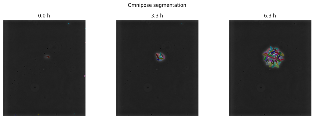
See what the model did#
Never trust a segmentation you have not looked at.
render_segmentation_mask() paints the masks over the image and,
as always, returns a source — so it composes with the annotation and video
helpers from tutorial 3.
import matplotlib.pyplot as plt
import numpy as np

from acia.viz import render_segmentation_mask

painted = render_segmentation_mask(src.to_rgb(), overlay, alpha=0.5)

fig, axes = plt.subplots(1, 3, figsize=(12, 4.2))
for ax, idx in zip(axes, [0, len(src) // 2, len(src) - 1], strict=True):
    ax.imshow(np.asarray(painted[idx].raw))
    ax.set_title(f"{src.timepoints[idx].to('hour'):~.1f}")
    ax.axis("off")
fig.suptitle("Omnipose segmentation")
fig.tight_layout()
plt.show()
from IPython.display import Video

from acia.viz import render_video

render_video(painted, "segmented.mp4", framerate=4)
Video("segmented.mp4", embed=True, width=420)
[rawvideo @ 0x2387f180] Stream #0: not enough frames to estimate rate; consider increasing probesize
Measure#
ExtractorExecutor turns the overlay into a tidy,
id-indexed DataFrame — one row per detection, one column per property. Because
the source is calibrated, areas come out in µm² and times in hours without any
further configuration.
from acia.analysis import (
    AreaEx,
    BoundaryClosenessEx,
    CircularityEx,
    ExtractorExecutor,
    FrameEx,
    PerimeterEx,
    TimeEx,
)

properties = ExtractorExecutor().execute(
    overlay,
    src,
    extractors=[
        FrameEx(),
        TimeEx(),
        AreaEx(),
        PerimeterEx(),  # CircularityEx is derived from area and perimeter,
        CircularityEx(),  # so PerimeterEx must come before it
        BoundaryClosenessEx(),
    ],
)

print(properties.head())
print()
print("units:", properties.attrs["units"])
    frame  time      area  perimeter  circularity  boundary_closeness
id
1     0.0   0.0  0.705024      3.888     0.586086               2.808
2     0.0   0.0  0.305856      2.592     0.572080               0.000
3     0.0   0.0  0.165888      2.016     0.512913               0.000
4     0.0   0.0  2.286144      7.056     0.577027              29.520
5     0.0   0.0  2.073600      6.768     0.568871              29.304

units: {'frame': '1 dimensionless', 'time': 'hour', 'area': 'micrometer ** 2', 'perimeter': 'micrometer', 'circularity': 'dimensionless', 'boundary_closeness': 'micrometer'}
Throw out the artefacts#
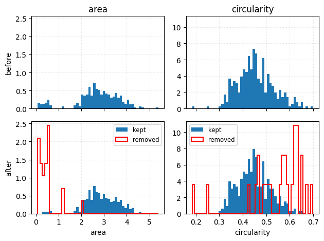
Real segmentations contain debris and merged blobs.
apply_cell_filters() takes the measured table and a list
of filters, with thresholds in physical units — which is the whole reason we
bothered with calibration.
from acia.segm.filter import AreaFilter, BoundaryClosenessFilter, apply_cell_filters

filters = [
    # a C. glutamicum cell is roughly 1-3 um^2; anything far below that is debris
    AreaFilter(vmin=0.3 * ureg.micrometer**2, vmax=10 * ureg.micrometer**2),
    # a cell clipped by the edge of the image has a meaningless area
    BoundaryClosenessFilter(min_distance=1 * ureg.micrometer),
]

filtered_overlay = apply_cell_filters(overlay, filters, properties=properties)

print(
    f"{len(overlay)} detections -> {len(filtered_overlay)} kept "
    f"({len(overlay) - len(filtered_overlay)} removed)"
)
346 detections -> 319 kept (27 removed)
plot_property_histograms() shows the before and
after distributions together, so you can see what a threshold actually did rather
than guessing.
from acia.analysis.properties import plot_property_histograms

properties_after = ExtractorExecutor().execute(
    filtered_overlay,
    src,
    extractors=[FrameEx(), TimeEx(), AreaEx(), PerimeterEx(), CircularityEx()],
)

plot_property_histograms(
    properties,
    ["area", "circularity"],
    df_after=properties_after,
    show_removed=True,
)
plt.show()
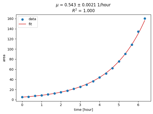
The growth rate#
extract_growth() does the last step in one call: it
aggregates total cell area per timepoint, fits an exponential model, and returns
the table, the fit result and a figure.
from acia.analysis import extract_growth

table, result, figure = extract_growth(filtered_overlay, src, time_unit="hour")

print(table.head())
print()
print("growth rate  :", result.growth_rate)
print("doubling time:", result.doubling_time)
print("R^2          :", round(result.r_squared, 4))
plt.show()
    frame      time      area
id
1     0.0  0.000000  0.705024
4     0.0  0.000000  2.286144
5     0.0  0.000000  2.073600
10    1.0  0.333333  0.580608
14    1.0  0.333333  2.788992

growth rate  : 0.5427718663757394 / hour
doubling time: 1.2770506791155367 hour
R^2          : 0.9997
Where to go next#
You now have the full loop: open → slice → visualize → segment → measure → filter → quantify.
Tracking and lineages. Add a tracker (
TrackastraTracker,UltrackTracker,LaptrackTracker,PyUATTracker) to follow individual cells through divisions, then plot lineage trees and per-cell doubling times.A different backend. Replace
CellposeSAMSegmenterwithCellposeSAMSegmenter(a strong generalist, but far heavier on CPU),CellposeSegmenter,CPNSegmenterorYOLOSegmenter— same call signature, different environment.Scale it up.
acia.analysis.scale()runs this notebook once per sequence across hundreds of positions; see Scaling a notebook over many sequences.Real experiments. The acia-workflows collection has complete published analyses — growth-rate quantification, fluorescence co-culture, single-cell oxygen response — built on exactly these pieces.