3. Look at your data

Before you segment anything, look at it. This notebook covers the three ways acia shows you a sequence: an interactive viewer inside Jupyter, static figures, and an annotated video with a scale bar and a clock.

# On Colab (or any fresh environment) this installs acia.
# Locally, if you already have acia installed, it is a no-op.
try:
    import acia  # noqa: F401
except ImportError:
    %pip install -q acia

from pathlib import Path
from urllib.request import (
    HTTPBasicAuthHandler,
    HTTPPasswordMgrWithDefaultRealm,
    build_opener,
    install_opener,
    urlretrieve,
)

# A public ownCloud share. The share token acts as the username, so single
# frames can be fetched over WebDAV instead of downloading the whole 800-frame,
# ~800 MB archive.
SHARE = "D0A9ftcpqwKm1Rq"
BASE = "https://fz-juelich.sciebo.de/public.php/webdav"
SEQUENCE = Path("data/colony")

N_FRAMES = 20  # of 800 available
FRAME_STEP = 20  # every 20th frame -> 20 minutes between the frames we keep

mgr = HTTPPasswordMgrWithDefaultRealm()
mgr.add_password(None, BASE, SHARE, "")
install_opener(build_opener(HTTPBasicAuthHandler(mgr)))

SEQUENCE.mkdir(parents=True, exist_ok=True)
for i in range(N_FRAMES):
    name = f"t{i * FRAME_STEP:04d}.tif"
    target = SEQUENCE / name
    if not target.exists():
        urlretrieve(f"{BASE}/00/{name}", target)

print(SEQUENCE, "->", len(list(SEQUENCE.glob("*.tif"))), "frames (~1 MB each)")

data/colony -> 20 frames (~1 MB each)

Load and shrink

We attach the acquisition’s calibration right away — 0.072 µm per pixel — because the scale bar and the timestamp need it. The frames on disk are every 20th frame of a 1 minute acquisition, so the interval for this source is 20 minutes. Tutorial 4 goes into what else that buys you.

Then we subsample again. 20 frames is not much, but the habit matters: everything below gets twice as cheap for free.

from acia import ureg
from acia.segm.open import open_sequence

full = open_sequence(SEQUENCE).position(0)
full = full.with_pixel_size(0.072 * ureg.micrometer).with_frame_interval(
    20 * ureg.minute
)

src = full[::2]  # every 2nd frame of the 20 we downloaded

print(f"{len(full)} frames -> {len(src)} frames")
print("pixel size    ", src.pixel_size)
print("timepoints    ", src.timepoints)

20 frames -> 10 frames
pixel size     0.072 micrometer
timepoints     [  0  40  80 120 160 200 240 280 320 360] minute

Note that the calibration followed the slice: the source interval is 20 minutes, so src.timepoints steps in 40 minute increments rather than silently staying at 20.

The interactive viewer

Every source in acia mixes in JupyterVisualizationMixin, so making the last expression of a cell a source gives you a viewer with a frame slider and channel toggles:

src

That is genuinely interactive — it needs a running kernel and ipywidgets, so it works in JupyterLab and on Colab but cannot be captured in this static page. Try it in your own session; it is the fastest way to scrub through a sequence.

The rest of this notebook uses static rendering, which works everywhere.

A contact sheet

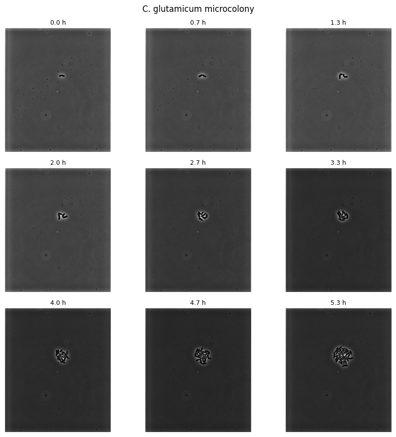
For a quick overview of the whole time course, matplotlib is hard to beat.

import matplotlib.pyplot as plt
import numpy as np

fig, axes = plt.subplots(3, 3, figsize=(9, 9))

for idx, ax in enumerate(axes.ravel()):
    ax.imshow(np.asarray(src[idx].raw).squeeze(), cmap="gray")
    ax.set_title(f"{src.timepoints[idx].to('hour'):~.1f}", fontsize=9)
    ax.axis("off")

fig.suptitle("C. glutamicum microcolony")
fig.tight_layout()
plt.show()

Grayscale to RGB

to_rgb() turns any source into a three-channel one. On a single-channel sequence it simply replicates the channel; on a multi-channel sequence you can map each channel to a colour, which is how fluorescence composites are built.

rgb = src.to_rgb()

print("channels:", src.num_channels, "->", rgb.num_channels)
print("frame shape:", np.asarray(rgb[0].raw).shape)

# multi-channel example (not executed -- our sample has one channel):
#   composite = two_channel_src.to_rgb(colors={0: "green", 1: "magenta"})

channels: 1 -> 3
frame shape: (1094, 938, 3)

Scale bar and clock

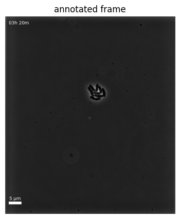
render_scalebar() and render_time() each take a source and return a new source with the annotation burned in. Because they return sources, they chain — and because they are lazy, chaining them costs nothing until frames are pulled.

The scale bar is specified in physical units, which is exactly why the calibration mattered.

from acia.viz import render_scalebar, render_time

annotated = render_scalebar(
    rgb,
    xy_position=(20, 1040),
    size_of_pixel=src.pixel_size,
    bar_width=5 * ureg.micrometer,
    bar_height=1 * ureg.micrometer,
)
annotated = render_time(
    annotated,
    xy_position=(20, 20),
    timepoints=list(src.timepoints),
    time_format="{H:02}h {M:02}m",
)

plt.figure(figsize=(5, 5))
plt.imshow(np.asarray(annotated[len(annotated) // 2].raw))
plt.axis("off")
plt.title("annotated frame")
plt.show()

Export a video

render_video() writes the sequence to a file. It is the last step of most workflows and, on long sequences, often the slowest — one more reason to subsample while you are still iterating.

from pathlib import Path

from acia.viz import render_video

render_video(annotated, "sequence.mp4", framerate=4)

print("wrote sequence.mp4:", Path("sequence.mp4").stat().st_size // 1024, "KiB")

wrote sequence.mp4: 352 KiB

[rawvideo @ 0x1f45f180] Stream #0: not enough frames to estimate rate; consider increasing probesize

from IPython.display import Video

Video("sequence.mp4", embed=True, width=420)

For finer control over codec and quality there is VideoExporter2, a context manager with ready-made presets:

from acia.viz import VideoExporter2

with VideoExporter2.default_h264("out.mp4", framerate=10) as exporter:
    for frame in annotated:
        exporter.write(frame.raw)

default_vp9, fast_vp9, default_h264 and default_h265 cover the usual trade-offs between file size, encoding time and browser support.

What you learned

• Any source displays as an interactive viewer in Jupyter — just put it last in a cell.

• to_rgb() produces displayable three-channel frames, with per-channel colours for composites.

• render_scalebar() and render_time() return new sources, so annotations chain lazily; the scale bar is in physical units.

• render_video() writes the result out, and VideoExporter2 gives you codec control.

Next: 4. Calibration and units — why pixel_size is worth setting, and what it does to your results.